You may have heard of iron–sulfur clusters as representative systems that challenge standard quantum-chemical methods. They are also increasingly used as targets for benchmarking quantum algorithms and for estimating the resources those algorithms require [1–5]. Among them, the [2Fe–2S] cluster is probably the simplest. Following Refs. [6, 7], this note works through the construction of an active-space Hamiltonian for the oxidized dimer [Fe₂S₂(SCH₃)₄]²⁻. It is a pedagogical tutorial written for my own learning and future sharing. It states what each step does and why it is justified; implementation details and all data are in the companion repository on my GitHub [8].
An active-space Hamiltonian replaces a molecule with a small many-electron problem. It contains only a few orbitals and electrons, mostly from the valence space, chosen to capture the essential reactive chemistry. Constructing it involves a sequence of standard steps: a parent calculation and its natural orbitals (Sec. 3), a frozen core (Sec. 4), localization (Sec. 5), selection (Sec. 6), and contraction of the closed shells (Sec. 7).
1. The active-space approximation
Partition an orthonormal set of orbitals into three blocks: a closed-shell block \(C\), an active block \(A\) with \(n_A\) orbitals, and a virtual block \(V\). The complete-active-space (CAS) wavefunction contains every configuration in which \(C\) is doubly occupied, \(V\) is empty, and the remaining \(N_A\) electrons are distributed over \(A\):
where \(\Phi_I^A\) runs over the determinants of \(N_\alpha\) up-spin and \(N_\beta\) down-spin electrons in \(A\).
Two properties organize everything that follows. First, the CAS energy depends only on the subspaces spanned by \(C\) and \(A\), not on the particular orbitals chosen within them: a unitary rotation within \(A\) maps the configuration space of Eq. (1) onto itself, and a rotation within \(C\) leaves the closed-shell density unchanged. Constructing an active space therefore means choosing two subspaces; the individual orbitals are a matter of convenience. Second, a rotation that mixes blocks in general changes the model.
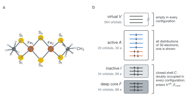
For [Fe₂S₂(SCH₃)₄]²⁻ [Fig. 1(a)] (186 electrons in 662 basis functions), the exact problem has \(\binom{662}{93}^2 \approx 5\times10^{230}\) determinants with \(N_\alpha = N_\beta\). The active space constructed below, CAS(30e,20o) [Fig. 1(b)], has \(\binom{20}{15}^2 = 2.4\times10^{8}\). Each iron is formally high-spin Fe(III), \(3d^5\), and the ground state is a singlet in which the two local spins \(S = 5/2\) are coupled antiferromagnetically. This ground state is not derived here; it is prior knowledge from experiment and earlier calculations [6], and it guides the choices below. Such a state is a superposition of many determinants with comparable weights.
2. Model and chemical choice of the active space
The geometry is the oxidized structure of Ref. [6]. The basis and Hamiltonian are those of the published model of Ref. [7]: the all-electron TZP-DKH basis [9] and the spin-free, one-electron exact two-component Hamiltonian (sf-X2C-1e) [10].
- All-electron basis. The core orbitals are treated explicitly (Sec. 4) rather than replaced by an effective core potential, so the Hamiltonian is defined for all 186 electrons.
- Scalar relativity. Relativistic corrections for iron are significant mainly in the core shells and, for valence chemistry, are dominated by the spin-free (scalar) terms. The sf-X2C-1e Hamiltonian obtains them by exactly decoupling the spin-free one-electron Dirac equation in the given basis. The result is a modified one-electron operator \(h\); the two-electron integrals, and all formulas below, are unchanged. The label "1e" means that the corresponding (picture-change) correction to the two-electron interaction is neglected. The TZP-DKH contractions were optimized for scalar-relativistic calculations [9].
- No spin–orbit coupling was used.
Assigning formal charges of −2 to each bridging sulfide and −1 to each methylthiolate leaves +3 on each iron. The active space should contain the orbitals whose ground-state occupations differ appreciably from 0 (unoccupied) and 2 (occupied). Here these are the ten Fe \(3d\) orbitals, which carry the unpaired electrons, and the sulfur orbitals that bond to them: the three \(3p\) orbitals of each bridging sulfide, through which the iron spins interact, and on each terminal sulfur the \(3p\) orbital directed along the S–Fe bond [11]. The cluster contains two irons, two bridging sulfides (Sb) and four terminal thiolate sulfurs (St) [Fig. 1(a)], so the chemical choice fixes the number of active orbitals.
The number of active electrons is not chosen separately. Once every orbital outside \(A\) is fixed as doubly occupied (\(n_C\) orbitals) or empty, the remaining electrons are active: \(N_A = N - 2n_C\). The natural orbitals of the parent (Sec. 3) comprise 88 nearly doubly occupied orbitals (\(1.998 < n \le 2\)) and ten singly occupied \(d\) orbitals (\(n = 1\)). The active space takes the ten \(d\) orbitals and ten of the nearly doubly occupied ones (the sulfur orbitals). The remaining \(n_C = 78\) are assigned occupation exactly 2; this is the closed-shell approximation of Eq. (1), not a property of the parent. Hence
The 156 electrons outside the active space occupy the 78 closed-shell orbitals. These are divided into a deep core \(F\) and an inactive set \(I\) [Table 1 and Fig. 1(b)]. In the CAS both are doubly occupied, so the division matters only for methods that later correlate the inactive electrons.
| Block | Orbitals | Electrons | Character |
|---|---|---|---|
| Deep core \(F\) | 44 | 88 | Fe and S \(1s,2s,2p\); C \(1s\) |
| Inactive \(I\) | 34 | 68 | Fe \(3s,3p\) (8); S lone pairs (10); S–C (4) and C–H (12) bonds |
| Active \(A\) | 20 | 30 | Fe \(3d\); bridging S \(3p\); Fe-directed terminal S \(3p\) |
| Virtual \(V\) | 564 | 0 | unoccupied |
3. A high-spin parent and its natural orbitals
In this construction the orbitals are fixed before the correlated calculation and taken from a single determinant, so the first question is which spin state that determinant should have. The singlet ground state is not a single determinant (Sec. 1); an unrestricted determinant with \(M_S = 0\) can only imitate it by breaking spin symmetry. The high-spin state is different. With all ten \(d\) electrons parallel there is exactly one way to place them in the ten \(d\) orbitals, so within the \(d\) shells the \(S = M_S = 5\) state is a single configuration. Moreover, in the spin-coupling picture of the dimer, the high-spin state and the singlet have the same orbital occupation (one electron in each \(d\) orbital) and differ only in how the local spins are coupled. A high-spin determinant therefore supplies orbitals suited to the whole manifold of spin states, with the \(d\) shells appearing as a block of singly occupied orbitals. The spin coupling is left to the correlated calculation.
The parent is an unrestricted Kohn–Sham determinant with the BP86 functional [12, 13], as in Ref. [6], with \(N_\alpha = 98\) and \(N_\beta = 88\).
An unrestricted determinant has different orbitals for the two spins. A single orthonormal set is obtained from the spin-summed density \(D = D^\alpha + D^\beta\) in the atomic-orbital (AO) basis with overlap \(S\):
The columns of \(C\) are the unrestricted natural orbitals (UNOs) and \(n\) their occupations. For a single unrestricted determinant the occupations have a simple structure. The singular value decomposition of the overlap between occupied \(\alpha\) and \(\beta\) orbitals defines corresponding orbitals \(a_i\) and \(b_i\) with \(\langle a_i|b_j\rangle = T_i\,\delta_{ij}\), \(0 \le T_i \le 1\). On each two-dimensional span \(\{a_i, b_i\}\), \(D\) acts as \(|a_i\rangle\langle a_i| + |b_i\rangle\langle b_i|\), with eigenvalues \(1 \pm T_i\), \(0 \le T_i \le 1\); each of the \(N_\alpha - N_\beta\) unpaired \(\alpha\) orbitals contributes an eigenvalue 1; all other eigenvalues vanish. The same overlaps determine the spin contamination:
Figure 2 shows the result for the Fe₂S₂ parent. The occupations fall into three sharply separated blocks: 88 nearly doubly occupied orbitals (\(\mathcal D\), \(1.998026 \le n \le 2\)), the ten singly occupied \(d\) orbitals (\(\mathcal O\), \(n = 1\) to within \(10^{-13}\)), and 564 nearly empty orbitals (\(\mathcal U\), \(n \le 0.001974\)). The small deviations from 2 and 0 occur in pairs \(1 \pm T_i\), as Eq. (4) requires. The companion repository assigns the blocks by the cutoffs \(n > 1.5\), \(0.5 \le n \le 1.5\) and \(n < 0.5\); because no occupation lies in the gaps between 0.002 and 0.998 or between 1.002 and 1.998, any cutoffs inside these gaps give the same blocks.
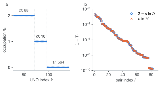
A broken-symmetry determinant behaves differently: its \(\alpha\) and \(\beta\) magnetic orbitals localize on different irons, their overlaps \(T_i\) are well below 1, and the \(d\) space appears as pairs of UNOs with occupations \(1 \pm T_i\) that differ from pair to pair, not as a degenerate block with \(n = 1\). The degeneracy matters in Sec. 5: rotations within a degenerate block return natural orbitals again.
A widely used rule, the UNO criterion [14], takes as active the UNOs whose occupations differ appreciably from 0 and 2, as judged by a threshold. Here any threshold inside the gaps above yields only the ten \(d\) orbitals of \(\mathcal O\); the ligand orbitals all lie in \(\mathcal D\) and must be selected by character.
4. The deep core
The occupations of Fig. 2 locate only half of the active space. The block \(\mathcal O\) contains exactly the ten Fe \(3d\) orbitals of Eq. (2). The ten sulfur orbitals, however, are nearly doubly occupied in the parent and lie in \(\mathcal D\), together with 78 orbitals that must remain closed-shell: core shells, bonding orbitals and other lone pairs. As natural orbitals these are delocalized mixtures, and since all have \(n \approx 2\), occupations cannot separate them. Sections 4–6 find the sulfur orbitals inside \(\mathcal D\) in three steps: remove the deep core, which is never active (this section); rotate the remaining occupied orbitals into localized orbitals with atomic identity (Sec. 5); and select by atomic character (Sec. 6). Each step is either a rotation within a block, which leaves the span of the block unchanged, or a choice of subspace. Figure 3 traces the orbitals through these steps.
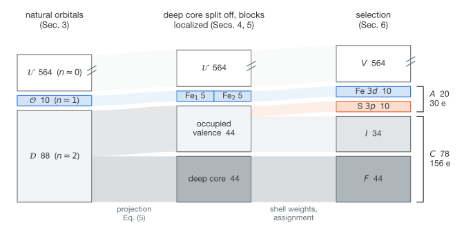
The deep core consists of the atomic inner shells, which are energetically separated from the valence and chemically inert. Removing them first also prevents the localization of Sec. 5 from mixing core and valence orbitals. The core is defined by projection. Let \(W\) be a set of orthonormalized AOs (here meta-Löwdin orbitals [15]) and \(W_\mathcal{C}\) the 44 of Fe and S \(1s,2s,2p\) and C \(1s\) character. With \(C_\mathcal{D}\) the orbitals of \(\mathcal D\),
Because both sets are orthonormal, the singular values of \(Q\) are the cosines of the principal angles [16] between the core-AO space and \(\mathcal D\), so \(0 \le \lambda_i \le 1\). The core orbitals are \(C_\mathcal{D} v_i\) for the 44 largest \(\lambda_i\). All 44 exceed 0.9998: the atomic core shells lie within 1° of the occupied space, so the deep core is well defined. Its orthogonal complement in \(\mathcal D\) is a 44-dimensional occupied-valence space.
The Fe \(3s\) and \(3p\) shells are not included in \(F\). Their radial extent overlaps that of the \(3d\) shell, so methods that correlate the inactive electrons should treat them as valence; in the CAS they are doubly occupied in either case.
5. Localization
A unitary rotation \(R\) within a block leaves the span of the block unchanged, and by Sec. 1 so does every model built from such spans. Localization uses this freedom to make orbitals that sit on few atoms. It does not require equal occupations; what equal occupations add is that the rotated orbitals are still natural orbitals. In the rotated basis the parent density matrix of a block is
so its off-diagonal elements are bounded by \(\max_k |n_k - \bar n|\), with \(\bar n\) the midpoint of the block's occupations. For \(\mathcal O\), where \(n = 1\) exactly, \(\gamma'\) stays diagonal. For the occupied orbitals of \(\mathcal D\) the bound is 0.001: the localized orbitals carry occupations between 1.998 and 2 and couplings of at most 0.001. These are discarded when the closed-shell orbitals are assigned occupation exactly 2 (Sec. 2), which is part of the CAS approximation rather than a consequence of localization. Mixing \(\mathcal D\) with \(\mathcal O\), by contrast, would produce orbitals with occupations between 1 and 2 coupled by up to 0.5, which no longer separate into closed-shell and open-shell orbitals.
The Pipek–Mezey method [17] maximizes
where \(q_X^{(i)}\) is a population of orbital \(i\) on atom \(X\). For a normalized orbital \(\sum_X q_X^{(i)} = 1\). For nonnegative populations, the sum of squares is then largest when the population is concentrated on few atoms. The choice of population belongs to the method; the companion repository uses Mulliken populations, which can be negative, so for them this reading is approximate. The deep core, the occupied valence and \(\mathcal O\) are localized separately (split localization [18]). The virtual block is not needed for the selection and is left unrotated.
To compare bases, a nonnegative population is more convenient. With orthonormal AOs \(W\) (here meta-Löwdin, as in Sec. 4), the coefficients \(P = W^{\mathsf T} S\, C\) satisfy \(\sum_\mu P_{\mu j}^2 = 1\) for each normalized orbital \(j\), and
are the fraction of orbital \(j\) on atom \(X\) and its effective number of atoms: \(N = 1\) for an orbital on a single atom and \(N = m\) for equal weights on \(m\) atoms. \(N\) serves here only as a diagnostic; it is not the quantity optimized in Eq. (7).
Figure 4 shows the effect. For comparison, each block is also represented by a delocalized basis: the eigenvectors of the spin-averaged Kohn–Sham operator restricted to the block, which resemble the canonical orbitals an SCF program returns. In the occupied valence these orbitals have \(N\) between 1.4 and 10.6 and mix lone pairs and bonds of different atoms; the Pipek–Mezey orbitals have \(1.0 \le N \le 2.0\) and are recognizable as Fe \(3s\) and \(3p\) shells, sulfur lone pairs, and S–C and C–H bonds. In \(\mathcal O\), each delocalized orbital is shared equally between the two equivalent irons (populations equal to within 0.01); localization separates the block into five orbitals on each iron, with a weight of at least 0.65 on their own iron and at most 0.01 on the other. Both bases span the same blocks.
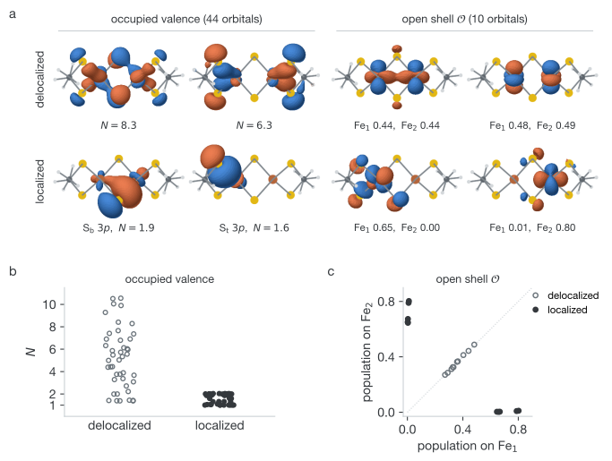
By Sec. 1, localization does not change any model by itself. It matters because the next step selects a subset of the localized orbitals, and the span of a subset depends on the rotation from which it is taken. The localization is therefore part of the definition of the active space.
6. Selection
Selection completes the active space, and its two halves play different roles. For the iron part there is nothing to choose: all ten orbitals of \(\mathcal O\) enter \(A\), and their span is fixed by the occupations of Sec. 3. Their Fe \(3d\) weights are used only to label which five belong to each iron. The sulfur part is a genuine choice: ten of the 44 occupied-valence orbitals must be taken, and since all have \(n \approx 2\), occupations cannot distinguish them; the selection uses atomic character. The other 34 form the inactive block \(I\).
Character requires a finer measure. Restricting the sum of Eq. (8) to one shell gives the shell weight
a well-defined fraction of orbital \(j\) on shell \(s\) of atom \(X\). (Mulliken populations in a nonorthogonal basis lack this property.) Three occupied-valence orbitals are assigned to each bridging sulfide, scored by \(w_{\mathrm S,3p}\), and one to each terminal sulfur, scored by the directional weight \(|\langle p_{\mathbf e}|\phi_j\rangle|^2\), where \(p_{\mathbf e} = \sum_m e_m\, p_m\) is the orthonormal \(3p\) function pointing along the unit vector \(\mathbf e\) from the sulfur to its iron. The assignment maximizes the total score subject to each orbital filling at most one slot (a linear assignment problem [19]). No energy enters the selection.
Figure 5(a) shows the composition of the twenty selected orbitals. Each has its intended character as the largest component, together with a substantial admixture of its bonding partner: S \(3p\) in the iron orbitals, and Fe \(3d\) (with some Fe \(4s\) and \(4p\)) in the sulfur orbitals. This admixture is Fe–S covalency. A label such as "terminal S \(3p\)" names the dominant character of an orbital, not a pure one.
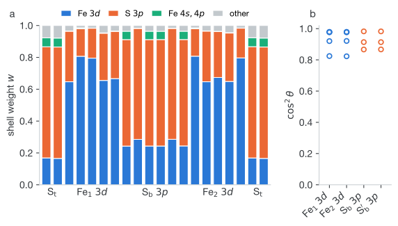
Because labels refer to individual orbitals, a separate test is needed to confirm that the subspace \(A\) contains every intended atomic direction. For a shell \((X,s)\), the matrix
(columns restricted to the active orbitals) has eigenvalues \(\cos^2\theta\), where \(\theta\) are the principal angles between the shell's atomic orbitals and \(A\). An eigenvalue near zero would signal an atomic direction missing from the active space. Figure 5(b) shows that all are far from zero: every \(d\) direction of each iron and every \(p\) direction of each bridging sulfide is represented in \(A\), and the remainder of each atomic orbital lies in orbitals outside \(A\).
7. The effective Hamiltonian
The orbitals enter the Hamiltonian through their coefficients. With real orthonormal orbitals \(\phi_p = \sum_\mu \chi_\mu C_{\mu p}\) in the AO basis \(\{\chi_\mu\}\), the integrals are transformed from the AO integrals,
where \(h^{\mathrm{AO}}\) is the one-electron operator (here sf-X2C-1e) and \((\mu\nu|\lambda\sigma)\) are electron-repulsion integrals in chemists' notation. For a basis of this size the four-index AO tensor is usually factorized first, for example by Cholesky decomposition, and the factors are transformed instead (step 07_ao_cholesky of the repository). The many-electron Hamiltonian is the physical one:
with \(\hat E_{pq} = \sum_\sigma a^\dagger_{p\sigma} a_{q\sigma}\). The Kohn–Sham exchange–correlation potential is not included. The two-electron term already contains exchange exactly and the correlated solver treats correlation explicitly; adding an approximate potential would count both twice. The density functional serves only to generate orbitals.
Let \(B\) be the set of orbitals doubly occupied in every configuration (\(B = F\cup I\) for the CAS). By the Slater–Condon rules, matrix elements between such configurations equal those of a Hamiltonian on the orbitals \(p, q \notin B\) with unchanged two-electron integrals and
The constant is the energy of the closed shells alone. The term \(2(pq|ii)\) is the Coulomb interaction with both electrons of closed-shell orbital \(i\), and \(-(pi|iq)\) the exchange with the one of the same spin. Three properties follow directly:
- \(h^{\mathrm{eff}}\) and \(E_\mathrm{core}\) depend on \(B\) only through its density \(\sum_{i\in B}|\phi_i\rangle\langle\phi_i|\), and are therefore invariant to rotations within \(B\) (Sec. 1).
- Contraction can be done in stages: freezing \(B_1\cup B_2\) is equivalent to freezing \(B_2\) in the Hamiltonian already contracted over \(B_1\).
- Orbitals that are empty in every configuration contribute no terms. Excluding \(V\) restricts the configurations, not the operator.
The constant \(E_\mathrm{core}\) is usually the dominant part of the total energy, and it is specific to the partition: a different choice of \(C\) and \(A\) moves energy between \(E_\mathrm{core}\) and the active-space energy, so only total energies can be compared between partitions. The result is commonly written as an integral file in the FCIDUMP format [20], which lists \(n_A\), \(N_A\) and \(2M_S\), the symmetry-distinct \((pq|rs)\), the elements of \(h^{\mathrm{eff}}\), and \(E_\mathrm{core}\). The file fixes only \(M_S\); the spin state is selected by the solver.
Reproduction. Each step corresponds to a directory of the companion repository [8]: parent and UNOs (02_parent_uks); core, localization and selection (03_localize_select); effective Hamiltonians (07_ao_cholesky, 08_full_hamiltonian). The correlated solution of the resulting Hamiltonian and its analysis are in the remaining directories.
References
- [1] M. Reiher, N. Wiebe, K. M. Svore, D. Wecker, and M. Troyer, Proc. Natl. Acad. Sci. USA 114, 7555 (2017).
- [2] Z. Li, J. Li, N. S. Dattani, C. J. Umrigar, and G. K.-L. Chan, J. Chem. Phys. 150, 024302 (2019).
- [3] J. Lee, D. W. Berry, C. Gidney, W. J. Huggins, J. R. McClean, N. Wiebe, and R. Babbush, PRX Quantum 2, 030305 (2021).
- [4] S. Lee et al., Nat. Commun. 14, 1952 (2023).
- [5] G. H. Low, R. King, D. W. Berry, Q. Han, A. E. DePrince III, A. White, R. Babbush, R. D. Somma, and N. C. Rubin, Phys. Rev. X 15, 041016 (2025); arXiv:2502.15882.
- [6] S. Sharma, K. Sivalingam, F. Neese, and G. K.-L. Chan, Nat. Chem. 6, 927 (2014).
- [7] Z. Li, Active-space model for iron–sulfur clusters (2026).
- [8] T. Jiang, Fe₂S₂ Hamiltonian reconstruction: a reusable worked example (2026).
- [9] F. E. Jorge, A. Canal Neto, G. G. Camiletti, and S. F. Machado, J. Chem. Phys. 130, 064108 (2009).
- [10] W. Liu and D. Peng, J. Chem. Phys. 131, 031104 (2009).
- [11] S. Sharma and G. K.-L. Chan, J. Chem. Phys. 136, 124121 (2012).
- [12] A. D. Becke, Phys. Rev. A 38, 3098 (1988).
- [13] J. P. Perdew, Phys. Rev. B 33, 8822 (1986).
- [14] P. Pulay and T. P. Hamilton, J. Chem. Phys. 88, 4926 (1988).
- [15] Q. Sun and G. K.-L. Chan, J. Chem. Theory Comput. 10, 3784 (2014).
- [16] Å. Björck and G. H. Golub, Math. Comput. 27, 579 (1973).
- [17] J. Pipek and P. G. Mezey, J. Chem. Phys. 90, 4916 (1989).
- [18] Z. Li and G. K.-L. Chan, J. Chem. Theory Comput. 13, 2681 (2017).
- [19] H. W. Kuhn, Nav. Res. Logist. Q. 2, 83 (1955).
- [20] P. J. Knowles and N. C. Handy, Comput. Phys. Commun. 54, 75 (1989).